Feature Extraction

Feature extraction is a crucial aspect of computer vision and image processing. It involves identifying specific structures within an image, such as points, edges, or objects, to gather information about its content. This process is typically performed at a low-level and serves as one of the initial steps in analyzing an image.

The goal of feature detection is to compute abstractions of image information and make local decisions at each pixel to determine the presence of a particular type of image feature. These detected features are subsets of the image and can take the form of single points, continuous curves, or connected parts. In this sections, we will explore some of the most popular algorithms for feature detection, also known as interest point detection algorithms.

Edge Detection Algorithms

An edge in an image refers to a significant change in pixel brightness, indicating a discontinuity in either the image intensity or its first derivative. There are several approaches to detecting edges, and we will briefly discuss some of the most commonly used methods, including:

• Prewitt Edge Detection
• Sobel Edge Detection
• Canny Edge Detection
• Laplacian of Gaussian (LoG)

Let's now delve into each of these methods.

Prewitt Edge Detection

Title: Prewitt Edge Detection in Computer Vision

Introduction: In the field of computer vision, edge detection plays a crucial role in identifying and extracting important features from images. Edge detection algorithms aim to locate the boundaries between different objects or regions within an image. One such algorithm is Prewitt Edge Detection, which is widely used due to its simplicity and effectiveness.

Explanation: Prewitt Edge Detection is a gradient-based edge detection algorithm that focuses on detecting edges by calculating the gradient magnitude of an image. It operates by convolving the image with two separate kernels, one for horizontal edges and the other for vertical edges. These kernels are known as Prewitt operators.

The Prewitt operator for horizontal edges is defined as:

\[ \begin{bmatrix} -1 & 0 & 1 \\ -1 & 0 & 1 \\ -1 & 0 & 1 \\ \end{bmatrix} \]

The Prewitt operator for vertical edges is defined as:

\[ \begin{bmatrix} -1 & -1 & -1 \\ 0 & 0 & 0 \\ 1 & 1 & 1 \\ \end{bmatrix} \]

To apply Prewitt Edge Detection, the image is convolved with both of these kernels. The horizontal kernel highlights vertical edges, while the vertical kernel highlights horizontal edges. The resulting convolutions are then combined to obtain the gradient magnitude of the image.

The gradient magnitude is calculated by taking the square root of the sum of the squared values of the horizontal and vertical convolutions at each pixel location. This magnitude represents the strength of the edge at that particular point.

Sobel Edge Detection

Another popular technique for edge detection is the Sobel operator, which is widely used due to its simplicity and effectiveness. This article aims to introduce and explain the Sobel edge detection algorithm, shedding light on its underlying principles and providing a practical example.

The Sobel operator is a gradient-based method that emphasizes edges by calculating the gradient magnitude of an image. It achieves this by convolving the image with two separate kernels: one for detecting horizontal edges and the other for vertical edges. These kernels are commonly referred to as the Sobel operators.

The horizontal Sobel operator, denoted as Gx, highlights vertical edges, while the vertical Sobel operator, denoted as Gy, emphasizes horizontal edges. By combining the results obtained from both operators, the Sobel algorithm computes the gradient magnitude, which represents the strength of the edges in the image.

The Sobel operator works by sliding the kernels over the image, calculating the gradient at each pixel. The gradient magnitude is then computed using the following formula:

Magnitude = sqrt(Gx^2 + Gy^2)

The resulting magnitude values are used to determine the presence of edges in the image. Higher magnitude values indicate stronger edges, while lower values represent smoother regions.

Overall, Sobel edge detection is a fundamental technique in computer vision that allows us to identify and extract edges from images. By leveraging the gradient magnitude, the Sobel operator provides a reliable method for feature extraction, enabling various applications such as object recognition, image segmentation, and more. Understanding and implementing the Sobel algorithm is essential for any AI practitioner delving into the field of computer vision.

Canny Edge Detection

Canny Edge Detection developed by John Canny in 1986, is widely used for detecting edges in images. It provides a robust and accurate way to identify boundaries between different objects or regions within an image.

Canny Edge Detection involves several steps to identify edges in an image. These steps are as follows:

1. Gaussian Smoothing: The first step is to apply a Gaussian filter to the image. This helps to reduce noise and smooth out any irregularities in the image.

2. Gradient Calculation: Next, the gradients of the image are calculated using the Sobel operator. This step helps to determine the intensity changes in different directions within the image.

3. Non-maximum Suppression: In this step, the algorithm identifies the local maxima in the gradient magnitude. It suppresses all other non-maximum values, ensuring that only the strongest edges are retained.

4. Double Thresholding: The image is then thresholded using two thresholds: a high threshold and a low threshold. Pixels with gradient magnitudes above the high threshold are considered strong edges, while those below the low threshold are considered non-edges. Pixels with gradient magnitudes between the two thresholds are considered weak edges.

5. Edge Tracking by Hysteresis: Finally, a process called edge tracking is performed to connect weak edges to strong edges. This helps to form continuous edges and eliminate any remaining noise.

Laplacian of Gaussian (LoG)

Laplacian of Gaussian (LoG) method combines the concepts of the Laplacian operator and Gaussian smoothing to accurately detect edges in an image. In this chapter, we will explore the theory behind LoG edge detection and provide an example to illustrate its application.

The Laplacian operator is a second-order derivative operator used to measure the rate of change of intensity in an image. It is particularly effective in detecting rapid changes, such as edges. However, the Laplacian operator is highly sensitive to noise, which can lead to false detections. To address this issue, the LoG method incorporates Gaussian smoothing.

Gaussian smoothing is a technique that applies a Gaussian filter to an image, which reduces noise and blurs the image slightly. By convolving the image with a Gaussian kernel, the LoG method effectively combines the benefits of both the Laplacian operator and Gaussian smoothing.

The LoG operator is defined as the Laplacian of a Gaussian function. It is obtained by convolving the image with the second derivative of a Gaussian function. The resulting image highlights regions of rapid intensity changes, which correspond to edges in the original image.

Corner detector

flat region, edge feature and corner feature

One commonly used algorithm for feature extraction is the corner detector. A corner is defined as the connecting point of two edges, where an edge represents a sharp change in image brightness. To detect corners, the corner detector algorithm analyzes a small window surrounding each pixel in an image. By moving the window slightly in a specific direction and measuring the change in pixel values, corners can be identified.

The detection process involves calculating the sum squared difference (SSD) between the pixel values before and after the window movement. If the SSD is large for motion in all eight directions, it indicates the presence of a corner. Specifically, a 3x3 pixel window around a pixel is examined to determine if it exhibits corner-like characteristics.

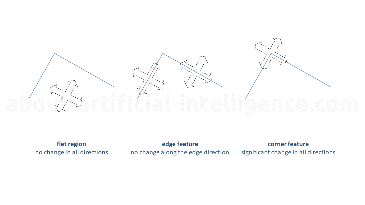
To illustrate the concept, consider the figure shown in corner-detection. This figure demonstrates the differences between a flat region, an edge feature, and a corner feature. In a flat region, there are no significant changes in brightness, resulting in a lack of corners. An edge feature, on the other hand, represents a sharp transition in brightness, indicating the presence of edges but not corners. Finally, a corner feature is characterized by the intersection of two edges, signifying the presence of corners.

By utilizing the corner detector algorithm, computer vision systems can effectively extract corner features from images. These extracted features can then be used for various applications, such as object recognition, image stitching, and motion tracking. The ability to accurately detect corners plays a vital role in enhancing the performance and capabilities of artificial intelligence systems in the field of computer vision.

Feature Descriptors

After detecting features in an image, the next step is to compute a descriptor for each feature. These descriptors are essential for characterizing the features and creating feature vectors. In simple terms, a feature descriptor is an algorithm that generates feature vectors, which are numerical representations of an image. Feature descriptors serve as a type of numerical footprint that encode valuable information into a sequence of numbers, enabling us to differentiate one feature from another. Ideally, feature descriptors should be invariant to image transformations, ensuring that we can still locate the feature even if the image undergoes alterations.

There are two main types of descriptors: local and global. Global descriptors define the shape and appearance of an entire object or a collection of points, while local descriptors focus on capturing shape and appearance within a local vicinity around a point.

Numerous feature descriptor algorithms exist, and we will now introduce some of the most well-known ones.

Scale-invariant feature transform (SIFT)

One widely used and highly effective feature extraction technique is Scale-Invariant Feature Transform (SIFT). SIFT was introduced by David Lowe in 1999 and has since become a cornerstone in various computer vision applications, including object recognition, image stitching, and 3D reconstruction.

SIFT is designed to extract distinctive and robust features from images, regardless of changes in scale, rotation, illumination, and viewpoint. It achieves this by identifying key points, known as keypoints or interest points, and describing them using local image gradients. These keypoints are selected based on their stability under different transformations, making them highly reliable for matching and recognition tasks.

The SIFT algorithm consists of four main steps:

1. Scale-space extrema detection: SIFT uses a Difference of Gaussian (DoG) approach to identify potential keypoints at multiple scales. By convolving the image with a series of Gaussian filters, it creates a scale-space pyramid. The DoG is then computed by subtracting adjacent scales to highlight regions with significant intensity changes.

2. Keypoint localization: In this step, potential keypoints are refined by eliminating low-contrast points and those located on edges. Additionally, keypoints that are poorly localized are discarded to ensure accurate feature extraction.

3. Orientation assignment: SIFT assigns an orientation to each keypoint to achieve invariance to image rotation. It computes the dominant gradient orientation in the local neighborhood of the keypoint and assigns it as the keypoint's orientation.

4. Feature descriptor generation: Finally, SIFT constructs a robust descriptor for each keypoint by considering the local image gradients in its vicinity. These descriptors capture the distribution of gradient orientations, providing a distinctive representation of the keypoint's appearance.

Example

Let's consider an example of using SIFT for object recognition. Suppose we have a database of images containing various objects, and we want to identify a specific object in a new image.

Using SIFT, we first extract keypoints and descriptors from both the database images and the new image. Then, we compare the descriptors of the keypoints in the new image with those in the database using techniques like nearest neighbor matching or RANSAC (Random Sample Consensus).

By finding the best matches between keypoints, we can determine the object's presence and even estimate its pose and location in the new image. This allows us to perform tasks such as object tracking, augmented reality, or image retrieval.

In summary, SIFT provides a powerful and robust feature extraction technique in computer vision, enabling machines to understand and interpret visual information with high accuracy and reliability. Its ability to handle scale, rotation, and viewpoint changes makes it a valuable tool in various AI applications.

Speeded Up Robust Feature (SURF)

introduce and explain XXXXXX in Computer Vision. give an example for it

SURF is a robust and efficient algorithm that allows for the detection and description of distinctive features in images, making it widely used in various computer vision applications.

SURF was introduced by Herbert Bay, Tinne Tuytelaars, and Luc Van Gool in 2006 as an improvement over the widely used SIFT (Scale-Invariant Feature Transform) algorithm. SURF is designed to be both faster and more robust than SIFT, making it suitable for real-time applications.

The key idea behind SURF is to use a combination of scale-invariant and rotation-invariant techniques to detect and describe features in an image. SURF achieves this by utilizing a novel interest point detector and a descriptor that captures the local image structure.

The interest point detector in SURF is based on the concept of the Hessian matrix, which measures the local intensity variations in an image. By analyzing the Hessian matrix, SURF identifies stable interest points that are invariant to scale changes and robust to noise. This allows SURF to detect features accurately even in the presence of image transformations such as rotation, scaling, and affine distortion.

Once the interest points are detected, SURF generates a descriptor for each point. The descriptor is computed by considering the intensity values in the neighborhood of the interest point. SURF employs a technique called the Haar wavelet response, which efficiently captures the local image structure. This descriptor is not only robust to changes in scale and rotation but also provides a compact representation of the feature, making it suitable for matching and recognition tasks.

Example

To illustrate the application of SURF, let's consider an example of object recognition in an image. Suppose we have a dataset of images containing various objects, and we want to identify a specific object in a given image.

Using SURF, we can first detect and extract the distinctive features from both the dataset images and the target image. These features could be corners, edges, or other salient points that are unique to each object.

Next, we compute the descriptors for these features using the SURF algorithm. The descriptors capture the local image structure around each feature point.

Finally, we can compare the descriptors of the features in the target image with those in the dataset images using techniques like nearest neighbor matching or machine learning algorithms. By finding the best matches, we can identify the object present in the target image.

The speed and robustness of SURF make it suitable for real-time object recognition tasks, such as augmented reality, image retrieval, and video analysis.

In conclusion, Speeded Up Robust Feature (SURF) is a powerful algorithm for feature extraction in computer vision. Its ability to detect and describe distinctive features accurately, even in the presence of image transformations, makes it a valuable tool in various artificial intelligence applications.

Binary Robust Independent Elementary Features (BRIEF)

Title: Binary Robust Independent Elementary Features (BRIEF) in Computer Vision

Introduction: In the field of computer vision, feature extraction plays a crucial role in enabling machines to understand and interpret visual data. One popular method for feature extraction is Binary Robust Independent Elementary Features (BRIEF). BRIEF is a fast and efficient algorithm that extracts distinctive and robust features from images, making it suitable for various computer vision tasks such as object recognition, image matching, and tracking.

Explanation: BRIEF is designed to capture local image properties that are invariant to changes in scale, rotation, and illumination. It achieves this by encoding the intensity comparisons between pairs of pixels within a local neighborhood. Unlike other feature extraction methods, BRIEF does not rely on gradient information or corner detection. Instead, it focuses on capturing the binary patterns formed by pixel intensity comparisons.

The BRIEF algorithm consists of the following steps:

1. Keypoint Detection: BRIEF first identifies keypoints in an image using a suitable method such as the Scale-Invariant Feature Transform (SIFT) or the Speeded-Up Robust Features (SURF).

2. Descriptor Generation: For each keypoint, BRIEF selects a set of pixel pairs within a local neighborhood. The pixel pairs are randomly chosen, and their locations are independent of the image content. BRIEF then compares the intensity values of these pixel pairs and encodes the results as binary strings.

3. Descriptor Matching: To compare two images, BRIEF computes the Hamming distance between the binary descriptors of their corresponding keypoints. The Hamming distance measures the number of bit differences between two binary strings. Keypoints with low Hamming distances are considered to be similar.

Example: Let's consider an example where BRIEF is used for image matching. Suppose we have two images, Image A and Image B, and we want to find matching keypoints between them.

1. Keypoint Detection: BRIEF detects keypoints in both Image A and Image B using the SIFT algorithm. These keypoints represent distinctive features in the images.

2. Descriptor Generation: For each keypoint in Image A, BRIEF selects a set of pixel pairs within a local neighborhood. Let's say it chooses 128 pixel pairs. BRIEF then compares the intensity values of these pixel pairs and encodes the results as a binary string of length 128.

3. Descriptor Matching: BRIEF computes the Hamming distance between the binary descriptors of the keypoints in Image A and Image B. It finds the keypoints with the lowest Hamming distances, indicating potential matches between the two images.

By using BRIEF, we can efficiently extract and match distinctive features between images, enabling tasks such as image recognition, object tracking, and image stitching.

Conclusion: Binary Robust Independent Elementary Features (BRIEF) is a powerful feature extraction algorithm in computer vision. Its ability to capture local image properties using binary comparisons makes it efficient and robust to various image transformations. BRIEF has been widely adopted in computer vision applications, contributing to advancements in artificial intelligence and image analysis.

Histogram of Oriented Gradients (HOG)

Another popular technique used for feature extraction is the Histogram of Oriented Gradients (HOG). HOG has proven to be highly effective in various computer vision tasks, including object detection, pedestrian detection, and facial recognition. This article aims to introduce and explain the concept of HOG in the context of computer vision.

The Histogram of Oriented Gradients is a feature descriptor that captures the local shape and appearance of an image. It is based on the observation that the distribution of gradient orientations within an image can provide valuable information about its content. By analyzing the gradients, HOG can effectively represent the edges and contours of objects, making it suitable for object recognition tasks.

The HOG algorithm consists of the following steps:

1. Image Preprocessing: The input image is first preprocessed to enhance its contrast and reduce noise. Common techniques include gamma correction, histogram equalization, and Gaussian smoothing.

2. Gradient Computation: The gradients of the image are calculated to capture the changes in intensity. This is typically done using the Sobel operator, which computes the gradient magnitude and orientation for each pixel.

3. Cell Formation: The image is divided into small cells, typically square regions. Each cell contains a fixed number of pixels, and the gradients within the cell are used to construct a histogram of gradient orientations.

4. Block Normalization: To account for variations in lighting and contrast, neighboring cells are grouped together to form blocks. The histograms within each block are then normalized to reduce the influence of these variations.

5. Descriptor Calculation: The final step involves concatenating the normalized histograms from all the blocks to form the HOG descriptor. This descriptor represents the image's local shape and appearance, capturing the distribution of gradient orientations.

Example

Let's consider the task of pedestrian detection using HOG. In this scenario, the goal is to identify pedestrians in images or video frames.

To apply HOG, we first preprocess the input image to enhance its contrast and reduce noise. Next, we compute the gradients of the image using the Sobel operator. The image is then divided into cells, such as 8x8 pixel regions. Within each cell, we construct a histogram of gradient orientations, capturing the local edge information.

To account for variations in lighting and contrast, neighboring cells are grouped together to form blocks. The histograms within each block are normalized, reducing the influence of these variations. Finally, the normalized histograms from all the blocks are concatenated to form the HOG descriptor.

By comparing the HOG descriptors of pedestrians with those of non-pedestrian regions, a machine learning algorithm can be trained to classify and detect pedestrians in new images or video frames.

In conclusion, the Histogram of Oriented Gradients is a powerful feature extraction technique in computer vision. It effectively captures the local shape and appearance of an image, making it suitable for various tasks such as object detection and recognition.

Binary Robust Invariant Scalable Keypoints (BRISK)

One popular method for feature extraction is the Binary Robust Invariant Scalable Keypoints (BRISK) algorithm. BRISK is a keypoint detector and descriptor that is widely used for various computer vision tasks, including object recognition, image stitching, and augmented reality.

BRISK is designed to detect and describe keypoints in an image, which are distinctive and robust to changes in scale, rotation, and illumination. The algorithm combines the advantages of both binary and gradient-based methods, making it efficient and effective in various scenarios.

The key idea behind BRISK is to use a binary descriptor that encodes the local intensity pattern around a keypoint. This binary descriptor is computed by comparing the intensity values of a set of sampled points in the neighborhood of the keypoint. By using binary comparisons, BRISK achieves computational efficiency while maintaining robustness to noise and illumination changes.

BRISK also incorporates scale invariance by employing a pyramid-like scale space representation. This allows the algorithm to detect keypoints at different scales, enabling it to handle objects of varying sizes. Additionally, BRISK utilizes a rotation-invariant pattern to ensure that keypoints are invariant to image rotations.

Example

To illustrate the application of BRISK, let's consider the task of object recognition. Suppose we have a dataset of images containing various objects, and we want to train an AI model to recognize these objects. We can use BRISK to extract keypoints and descriptors from these images, which will serve as the basis for matching and identifying objects.

For instance, let's say we have an image of a cat and another image of a dog. By applying BRISK, we can detect and describe keypoints in both images. The keypoints will capture distinctive features such as corners, edges, or texture patterns. The descriptors will encode the local intensity patterns around these keypoints.

During the recognition phase, the AI model can compare the keypoints and descriptors of an input image with those of the training images. By finding matches between the keypoints, the model can determine the object present in the input image. In this case, the model would identify whether the input image contains a cat or a dog based on the matches found using BRISK.