Reinforcement Learning

@fig:reinforcement-learning

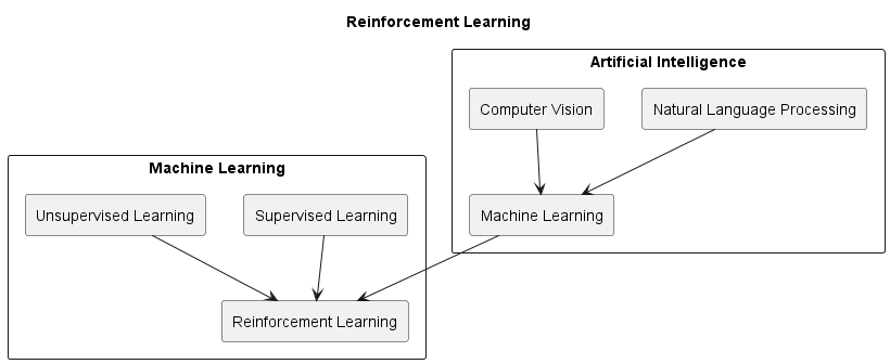
Reinforcement learning is a type of machine learning that focuses on developing algorithms that learn to make decisions through trial-and-error interactions with an environment. Unlike supervised learning, where a model is trained on labeled data, and unsupervised learning, where a model identifies patterns and relationships in unlabeled data, reinforcement learning is concerned with learning how to take actions in an environment to maximize a reward signal. This approach to machine learning has been used to develop AI systems that can play games, control robots, and even trade stocks. Reinforcement learning has become increasingly popular in recent years due to its ability to handle complex problems with no pre-defined solution and its potential to develop more human-like decision-making abilities.

Basic Case

In the most basic case, reinforcement learning (RL) is about an agent that determines the best strategy (policy) to achieve a goal (goal state) in an environment. In doing so, it can change from one state to another employing defined actions until it finally reaches the goal state. The approach is feasible through a model, which we will take a look at next.

In a simple RL model, an agent and its environment is given. The environment consists of a set S of states. The agent has a discrete set A of actions at its choice.

In a typical workflow of an RL model, the agent receives information on the present state of the environment s. The agent then selects a possible action (a) from set A of available actions. A reward or punishment (r) is given to the agent once the action is completed, and the agent receives the new state of the environment. The agent is now attempting to increase its utility (reward) in the long run by its actions. reinforcement-learning-model illustrates this simple workflow.

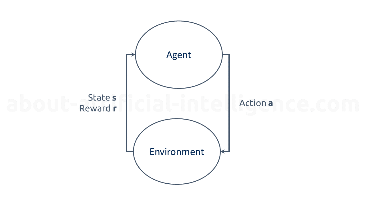
The environment's reaction to the agent's action influences the agent's choice of action in the next state. Over several thousands, hundreds of thousands, or even millions of iterations, the agent can approximate a relationship between its actions and the future expected utility in each state and thus behave optimally accordingly. In doing so, the agent is always in a dilemma between using its previously acquired experience on the one hand and exploring new strategies to increase reward on the other. This is called the \"exploration-exploitation dilemma\" (Yogeswaran & Ponnambalam, 2012).

Here are the basic terms for reinforcement learning:

Agent: The agent has to perform the actions in an environment and gets a reward for doing so.
Environment: The scenario that the agent must explore.
Action: Essentially, actions are the ways by which the agent interacts with and changes its environment.
Reward: Immediate feedback to an executed action.
State: The current state of the agent in the environment.
Policy: It is a strategy that an agent employs in achieving goals. It determines the actions that the agent takes depending on the state of the agent and the environment.
Value Function: The value function sets the value for a reward. A reward for reinforcement learning can be positive or negative.

To illustrate the concept behind the reinforcement learning approach, consider a tuple \((S,A,\pi)\), where:

\(S\): the set of states
\(A\): the set of actions
\(\pi\): a policy function \(\pi(s,a)\)

The policy function \(\pi(s,a)\) specifies the probability with which an agent in state \(s\) chooses action \(a\).

\[\pi(a|s) = Prob(a_t=a | s_t=s)\]

The goal of the reinforcement leaning approach is then to optimize this policy function. A practical example would be a two-dimensional maze as shown in the following figure:

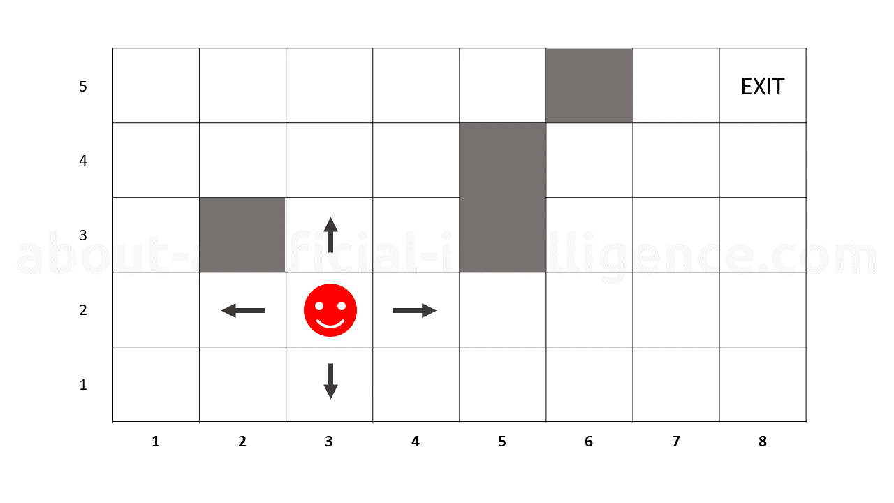
Reinforcement learning example: maze solver robot

In the maze-solver-robot a robot, which is currently in position (3, 2), must find the shortest path to the exit position. For each \((x,y)\) position, the robot would have the option to go up, down, right, or left. In this example, a state could be \(s = (x, y)\) and the actions up, down, right, left. The policy function \(\pi((3, 2), up)\) would return the probability that an agent in position (3, 2) would move \"up\".

The policy function returns the expected reward for a given state. Since it is not possible to predict what the expected reward will be the first time, the policy function is initialized with equal values for all state-action pairs.

In the simplest case, a policy function can be represented as a table. It can be viewed as a hash map that stores the state, action and probability. When searching for a "state + action" pair, the policy function returns the probability. The following table shows an example representation of the policy function for maze solver robot example.

State	Action	Probability
(1,1)	Up	0.2
(1,1)	Down	0.0
(1,1)	Right	0.8
(1,1)	Down	0.0
...	...	...
(3,2)	Up	0.1
(3,2)	Down	0.1
(3,2)	Right	0.7
(3,2)	Down	0.1
...	...	...

Table: Reinforcement learning example: policy function

Markov Chain

Markov Chain is a mathematical framework that forms the basis of many reinforcement learning algorithms. A Markov Chain is a stochastic process that satisfies the Markov property, which states that the future state of the process depends only on the current state and not on the past states. In other words, the future is independent of the past given the present state.

Markov chains allow us to predict future states based on probabilities of their occurrence, with the unique feature that the likelihood of the next state depends solely on the current state. This means that past states have no impact on the prediction of future states, making the Markov chain a "memoryless" model. A Markov Decision Process (MDP) is an extension of Markov chains in which an agent makes decisions to achieve the highest reward. The agent navigates a set of states by choosing from a set of actions, with the resulting state being determined by probabilities based on the current state and chosen action. The reward for each transition is determined by the initial and final states, as well as the action taken. The agent begins in a start state and ends in various final states where no further actions can be taken. The goal of an MDP is to find a policy that assigns the best action for each state to maximize overall profit. The mathematical foundation of reinforcement learning is the Markov Decision Process.

An MDP is a 5-tuple \((S, A, R, P, G)\):

S: the set of states
A: the set of actions
R: \(S \times S \times A \to A\): a reward function
P: \(S \times S \times A \to [0,1]\): the conditional transition probability
G: \(G \subseteq S\) the set of target states with \(z \in G\) a target state

In addition to the transition probability \(p\), each state transition is also assigned a reward. The goal of the action planner is to find a strategy \(\pi: S \to A\) which achieves a target state and maximize the expected reward \(r\).

Let \(R\) the reward function that assigns to each state \(s \subseteq S\) the expected reward to a target state \(z \subseteq G\). A strategy \(\pi\) is defined as follows:

\[\pi_{R}(s) = {argmin}_{a \in A} \sum_{s' \in S} P(s'|s,a)R(s,a,s')\]

Under stochastic conditions, a usuall MDP is a valuable model for action planning. On the other hand, the model has two flaws: first, the actions are carried out in a sequential manner, and second, all actions take place in real time. In practice, this is impossible since activities require time, and parallel execution can be advantageous to boost efficiency in some cases. For example, one robot arm may be doing an action while the other is in the process of transitioning to a new state and is otherwise occupied. Reinforcement learning means that an agent interacts with the environment based on the MDP concept by being in a state where it has to choose an action . After performing action a in the environment, the agent in state s will move to the next state \(s'\) with transition probability p. For the transition, the agent is rewarded with \(r\), which can be seen as a punishment if the \(r\) value is negative.

Algorithms

Reinforcement learning is a class of machine learning algorithms that enables agents to learn optimal decision-making policies through interactions with their environment. RL algorithms can be broadly categorized into three main types: model-based, model-free, and actor-critic methods.

Model-based methods: Model-based RL algorithms learn a model of the environment dynamics, such as the transition probabilities and reward function, and use this model to determine an optimal policy. The agent first learns the model by observing the environment, and then uses the model to plan ahead and choose the best action. Examples of model-based algorithms include dynamic programming.
Model-free methods: Model-free RL algorithms, on the other hand, do not learn a model of the environment dynamics, but instead directly learn an optimal policy from trial-and-error experience. These methods are generally more scalable and can handle larger state and action spaces, but may require more samples to learn a good policy. Examples of model-free algorithms include Monte Carlo methods, Q-learning and SARSA.
Actor-critic methods: Actor-critic methods combine elements of both model-based and model- free approaches. In actor-critic methods, the agent maintains both an actor and a critic component. The actor component is responsible for selecting actions based on the current policy, while the critic component evaluates the quality of the policy by estimating the expected cumulative reward. By using both components, actor-critic methods can learn an optimal policy more efficiently and effectively than either model-based or model-free methods alone.

Dynamic programming

Dynamic programming is a powerful algorithmic technique for solving sequential decision-making problems known as Markov decision processes (MDPs). In reinforcement learning, dynamic programming is used to find the optimal policy for an MDP by iteratively evaluating and improving the value function or the Q-function of the policy.

The basic idea behind dynamic programming is to break down the complex problem of finding the optimal policy into smaller subproblems that can be solved independently and then combined to obtain the overall solution. This is achieved by the principle of optimality, which states that an optimal policy has the property that whatever the initial state and the initial decision are, the remaining decisions must constitute an optimal policy with regard to the state resulting from the first decision.

Dynamic programming algorithms typically involve two key steps:

Value iteration
Policy iteration

In value iteration, the algorithm starts with an initial estimate of the value function or Q-function and iteratively updates it until it converges to the optimal value function or Q-function. The update rule is based on the Bellman equation, which expresses the value of a state or a state-action pair in terms of the immediate reward and the value of the next state or next state-action pair. The convergence of value iteration is guaranteed under certain conditions, such as the assumption that the MDP is finite and stationary.

In policy iteration, the algorithm starts with an initial policy and iteratively improves it by evaluating and optimizing its value function or Q-function. The evaluation step involves computing the value function or Q-function of the policy by solving the Bellman equation for each state or state-action pair. The optimization step involves selecting the best action for each state based on the current value function or Q-function. The policy iteration algorithm converges to the optimal policy under certain conditions, such as the assumption that the MDP is finite and stationary and the policy space is finite.

Dynamic programming has several advantages as a reinforcement learning algorithm. It is computationally efficient, since it avoids redundant computations by exploiting the recursive structure of the Bellman equation. It can handle large and complex MDPs, since it decomposes the problem into smaller subproblems that can be solved independently. It can handle stochastic and non- deterministic MDPs, since it takes into account the probabilities of transitions and the randomness of rewards. Dynamic programming is also widely used as a theoretical tool for analyzing and understanding the properties of MDPs and their solutions.

Monte Carlo methods

Monte Carlo methods are a class of reinforcement learning algorithms that use experience samples obtained from simulation or interaction with an environment to estimate the value function or the Q-function of a policy. Unlike dynamic programming, which requires a complete model of the MDP, Monte Carlo methods can learn from experience without making any assumptions about the transition probabilities or the reward function.

The basic idea behind Monte Carlo methods is to estimate the value of a state or a state-action pair by averaging the returns obtained from samples of episodes that start from that state or that state- action pair and follow the current policy. The return is defined as the sum of discounted rewards obtained from the starting time step to the terminal time step of the episode. By averaging over multiple samples, the Monte Carlo method can obtain an unbiased estimate of the true value, with a decreasing variance as the number of samples increases.

There are two main variants of Monte Carlo methods: on-policy and off-policy. On-policy Monte Carlo methods, such as every-visit Monte Carlo and first-visit Monte Carlo, estimate the value of the policy that is used to generate the samples. This means that the policy must be stochastic and explore all the possible states and actions in order to obtain accurate estimates. Off-policy Monte Carlo methods, such as importance sampling Monte Carlo and weighted importance sampling Monte Carlo, estimate the value of a different policy from the one used to generate the samples. This means that the policy can be deterministic or greedy, and the samples can be reused to estimate multiple policies.

Monte Carlo methods have several advantages and disadvantages as a reinforcement learning algorithm. They are model-free, meaning that they can learn directly from experience without requiring a model of the MDP. They can handle stochastic and non-deterministic MDPs, since they use samples of episodes that can have different trajectories and outcomes. They can also handle episodic and non- episodic tasks, since they can estimate the value of a state or a state-action pair based on the returns obtained from any subset of episodes that visit that state or that state-action pair. However, Monte Carlo methods can be computationally expensive, especially for large MDPs or long episodes, since they require a large number of samples to obtain accurate estimates. They can also suffer from high variance or bias, depending on the sampling distribution and the importance weighting scheme used.

Q-learning

Q-learning is a popular reinforcement learning technique that enables an agent to learn an optimal policy by iteratively exploring and exploiting the state-action space of a given environment. The approach is based on the concept of Q-values, which represent the expected cumulative reward of taking a particular action in a given state. The Q-learning algorithm involves estimating these values through an iterative update process that seeks to converge to the optimal policy that maximizes the expected cumulative reward over time.

The Q-learning algorithm is often used in scenarios where the agent has limited prior knowledge about the environment and must learn to take actions to achieve a particular goal. This is achieved by maintaining a Q-table, which stores the estimated Q-values for each state-action pair. At each iteration of the algorithm, the agent observes the current state of the environment and selects an action based on an exploration-exploitation trade-off strategy. The agent then receives a reward signal and updates the corresponding Q-value in the Q-table according to the Q-learning update rule. The update rule involves a weighted average of the current Q-value and the expected reward of taking the selected action in the next state, discounted by a factor that accounts for the long-term impact of the action.

Q-learning is a model-free reinforcement learning algorithm that learns the optimal action-value function \(Q(s, a)\) for an MDP. The Q-value represents the expected cumulative reward for taking action a in state s and following the optimal policy thereafter. The algorithm updates the Q-values iteratively based on the observed state transitions and rewards, using the following update rule:

\[ Q(s, a) \leftarrow Q(s, a) + \alpha \cdot (r + \gamma \cdot \max_{a'} Q(s', a') - Q(s, a)) \]

where Q(s, a) is the current estimate of the Q-value for state \(s\) and action \(a\), \(α\) is the learning rate that determines the influence of new information on the Q-value, \(r\) is the observed reward for taking action \(a\) in state \(s\) and transitioning to state \(s'\), \(\gamma\) is the discount factor that determines the importance of future rewards, and \(max(Q(s', a'))\) is the maximum Q-value over all possible actions \(a'\) in state \(s'\).

The Q-learning algorithm starts with an initial Q-value function, and repeatedly interacts with the environment by selecting actions based on an exploration strategy such as \(\varepsilon-greedy\), which chooses the optimal action with probability \(1 - \varepsilon\) and a random action with probability \(\varepsilon\). At each time step, the algorithm observes the current state s, selects an action a based on the exploration strategy, receives a reward \(r\), and observes the next state \(s'\). The Q-value for the state-action pair \((s, a)\) is then updated using the above formula.

The Q-learning algorithm converges to the optimal Q-value function \(Q*\) under certain conditions, such as the assumption that the MDP is stationary, deterministic, and has finite state and action spaces. The optimal policy can be derived from the optimal Q-value function by selecting the action with the highest Q-value in each state. The Q-learning algorithm is widely used in various applications, such as robotics, gaming, and control systems, due to its simplicity, effectiveness, and scalability.

One of the main advantages of Q-learning is its ability to learn an optimal policy without requiring a model of the environment or explicit knowledge of the reward function. This makes Q-learning suitable for complex real-world scenarios where the agent must learn from experience and adapt to changing environments. Additionally, Q-learning can handle continuous state and action spaces by using function approximation techniques, such as neural networks, to estimate the Q-values.

Despite its many advantages, Q-learning also has some limitations. One major issue is the problem of exploration, where the agent may become stuck in a suboptimal policy if it fails to explore all state-action pairs. Another challenge is the issue of overestimation, where the Q-values become inflated due to noise or incorrect estimates. Various modifications to the basic Q-learning algorithm have been proposed to address these issues, such as the use of exploration strategies, regularization techniques, and deep reinforcement learning methods.

Q-learning is a powerful reinforcement learning technique that has been used to develop intelligent agents in various domains, including robotics, game playing, and autonomous systems. By enabling agents to learn optimal policies through trial-and-error interactions with the environment, Q-learning has the potential to revolutionize the way we approach complex decision-making problems.

SARSA

SARSA (State-Action-Reward-State-Action) is a popular reinforcement learning (RL) algorithm that is widely used for learning optimal policies in sequential decision-making problems. In SARSA, an agent interacts with an environment by taking actions and receiving rewards in response, with the goal of maximizing the cumulative reward over time. SARSA is an on-policy algorithm, which means that it updates its policy while following it. This is in contrast to off-policy algorithms like Q-learning, which update their policy while following a different, fixed policy.

The SARSA algorithm is based on the principle of temporal difference learning, which involves updating the estimate of the value of a state-action pair based on the difference between the estimated value of the current state-action pair and the estimated value of the next state-action pair. In SARSA, the agent learns the Q-function, which is a function that maps a state-action pair to an estimate of its expected cumulative reward.

The Q-function can be defined as follows:

\[ Q(s, a) = E[R_t+1 + \gamma \cdot Q(s_t+1, a_t+1) | s_t = s, a_t = a] \]

where \(s\) is the current state, \(a\) is the action taken, \(R_t+1\) is the reward received in response to the action, \(s_t+1\) is the next state, \(a_t+1\) is the next action, \(\gamma\) is a discount factor that determines the weight given to future rewards, and \(E[\dots]\) denotes the expected value.

The SARSA algorithm updates the Q-function estimate based on the observed rewards and actions taken by the agent. The update rule for SARSA is as follows:

\[ Q(s_t, a_t) \leftarrow Q(s_t, a_t) + \alpha \cdot [R_t+1 + \gamma \cdot Q(s_t+1, a_t+1) - Q(s_t, a_t)] \]

where \(\alpha\) is the learning rate, which determines the weight given to the new information compared to the previous estimate.

In comparison to Q-learning, SARSA updates the Q-function estimate based on the next action taken by the agent, rather than the maximum Q-value over all possible actions. This makes SARSA an on-policy algorithm, because the policy being updated is the same one that is being used to generate the data. In contrast, Q-learning is an off-policy algorithm, because it updates the Q-function estimate based on the maximum Q-value over all possible actions, which is generated by a different, fixed policy.

SARSA is a flexible and widely used RL algorithm that can be used to solve a variety of sequential decision-making problems. Its on-policy nature and ability to handle stochastic environments make it a powerful tool for a wide range of applications.