Supervised Learning

Supervised learning is a type of machine learning where an algorithm is trained to predict an output or label given a set of inputs or features. The algorithm is provided with a labeled dataset, which consists of input-output pairs, where the output is also known as a label or a target variable. The algorithm learns from this dataset by finding patterns and relationships between the inputs and outputs, and then uses this learned model to predict the output for new inputs.

Supervised learning is commonly used in a wide range of applications, such as image recognition, speech recognition, natural language processing, and predictive modeling. It is the most widely used type of machine learning, and it's the starting point for most machine learning practitioners.

Supervised learning is widely used in various applications, such as image recognition, speech recognition, natural language processing, and predictive modeling. It is the most widely used type of machine learning, and is the starting point for most machine learning practitioners.

In this section we will first introduce the process of supervised learning. Afterward, we will delve into the core concepts of supervised learning, encompassing various algorithmic and model approaches, such as Naive Bayes, Maximum Entropy, Decision Trees, Support Vector Machines (SVM), Logistic Regression, K-Nearest Neighbors (KNN), and Random Forests. Furthermore, we will engage in a discussion surrounding significant challenges and factors to consider in the context of supervised learning, which includes the issues of overfitting, underfitting, and the selection of appropriate evaluation metrics.

Supervised Learning Process

Understanding the intricacies of the learning process in supervised machine environments is critical to realising the full potential of this widely used paradigm.

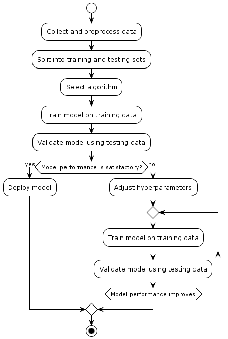
Supervised Machine Learning Process

supervised-machine-learning-process represents the process of supervised machine learning in a simple and visual way. Here's an explanation of each step:

1. Collect and preprocess data: In this step, you gather the data that you'll use to train and test your machine learning model. This data might include features (inputs) and corresponding labels (outputs). Before using the data, you might need to clean it, handle missing values, and convert it into a suitable format.

2. Split into training and testing sets: The collected data is divided into two sets: the training set and the testing set. The training set is used to teach the machine learning model patterns and relationships within the data. The testing set is used to evaluate how well the model performs on new, unseen data.

3. Select algorithm: Choose an appropriate machine learning algorithm that matches the problem you're trying to solve. Different algorithms have different characteristics and are suited for different types of tasks (e.g., regression, classification).

4. Train model on training data: Using the training set, the selected algorithm is trained to learn patterns and relationships in the data. The algorithm adjusts its internal parameters to minimize the difference between its predictions and the actual labels in the training set.

5. Validate model using testing data: The trained model is then tested on the testing set, which it has never seen before. This helps you assess how well the model generalizes to new data. You measure its performance using various metrics, such as accuracy, precision, recall, etc.

6. Model performance satisfactory? This is a decision point. If the model's performance on the testing data is satisfactory and meets your requirements, you move on to the next step.

7. Deploy model: If the model performs well, you deploy it into real-world applications to make predictions on new, unseen data.

8. Adjust hyperparameters: If the model's performance is not satisfactory, you need to fine-tune it. This involves adjusting hyperparameters, which are settings that control the behavior of the learning algorithm.

9. Repeat training and validation: After adjusting the hyperparameters, you repeat the process of training the model on the training data and validating its performance on the testing data.

10. Repeat while model performance improves: You continue fine-tuning the model's hyperparameters and iterating through training and validation until the model's performance on the testing data starts to improve or reaches a desired level.

11. Stop: You stop the iterative process when the model's performance is considered satisfactory or when you've reached a predefined stopping point.

This iterative process of training, testing, and adjusting continues until the model performs well enough on the testing data, at which point it can be deployed for real-world predictions.

Core Concepts

Given a set of input data points \({x_1,...,x_m}\) associated to a set of output data \({y_1,...,y_m}\) the goal is to train a model that is able to predict \(y\) from \(x\).

The problem of supervised learning can be formulated as follows:

Given an unknown function \(g: \mathcal{X}\rightarrow \mathcal{Y}\) which is known as the ground truth and maps input instances \(x \in \mathcal{X}\) to output labels \(y \in \mathcal{Y}\), along with training data \(\mathbf{D} = {({x}_1,y_1),\dots,({x}_n, y_n)}\), the goal is to find a function \(h:\mathcal{X}\rightarrow\mathcal{Y}\) that approximates as closely as possible the correct mapping \(g\).

In the context of this discussion, the term "approximates as closely as possible" is defined by specifying a loss function, also known as a cost function, which assigns a particular value to the "loss" incurred when producing an incorrect label. The objective, in this case, is to minimize the expected loss. To calculate the distribution of \(\mathcal{X}\) and the ground truth function \(g:\mathcal{X}\rightarrow\mathcal{Y}\), empirical methods are employed, involving the collection of a substantial number of samples of \(\mathcal{X}\) along with their corresponding labels \(\mathcal{Y}\).

The choice of loss function depends on the type of label being predicted. For instance, in binary classification, a straightforward zero-one loss function suffices. This function assigns a loss of 1 to any incorrect labeling. Essentially, it corresponds to computing the accuracy of the classification procedure over a set of test data, with the objective being to maximize this accuracy.

From a probabilistic point of view, the supervised learning problem is to estimate a function \(f\) which is the probability of each possible output label \(y\) given a particular input instance \(x\):

\[p({y}|{x},\theta) = f({x};{\theta})\]

where the feature vector input is \(x\), and the function \(f\) is typically parametrized by some parameters \(\theta\).

Frequentist vs. Bayesian Inference

In the context of the supervised learning process, the third step, as previously mentioned, is titled as "Algorithm selection" and it plays a central role. This step involves the essential tasks of building, evaluating and perfecting a predictive model to ensure accurate predictions for new data. This multi-faceted endeavour involves finding the most appropriate model that is able to effectively capture the intricacies of the data and its relationship to the target variable.

The journey through this step involves several critical participants, including data pre-processing, careful algorithm selection, rigorous model training and thorough performance evaluation. Building a robust model also involves fine-tuning the hyperparameters, a careful process that aims to optimise the model's internal settings to improve its predictive performance.

One of the core concepts of supervised learning is the idea of a hypothesis or model, which is a set of mathematical equations or rules that define the relationship between the inputs and outputs. The goal of supervised learning is to find the best hypothesis that can accurately predict the output for new inputs. This process is often referred to as training or model fitting.

A solid grasp of Statistical Inference is fundamental for delving into the core concepts of Machine Learning, as numerous Machine Learning models are rooted in these principles.

Statistical inference is about gaining insights from data. Essentially, it involves approximating an unknown pattern by examining the resulting data. There are several approaches to computational learning theory, and the main differences arise from different interpretations of probability and different assumptions about how samples are generated. These different interpretations of probability lead to two different inference methods:

1. Frequentist Inference
2. Bayesian Inference

Frequentist inference treats probability as a representation of long-term relative frequency. This approach entails testing hypotheses by comparing observed and expected data under the null hypothesis, using metrics like p-values. If the p-value is exceedingly small, it suggests that the observed data significantly deviates from what's anticipated under the null hypothesis, prompting acceptance of the alternative hypothesis. The p-value quantifies the likelihood of observing data as extreme or more extreme than the observed data, assuming the null hypothesis holds.

Bayesian inference views probability as a measure of belief. This method involves updating an initial belief about a hypothesis using observed data, resulting in a posterior probability. This framework permits the integration of prior knowledge and subjective judgment into analysis. Moreover, it enables the quantification of uncertainty by employing probability distributions.

The core concept of Bayesian inference rests on the idea that the probability of event A given event B depends not solely on their relationship, but also on the individual probability of each event:

\[p(A|B) = \frac{p(B|A) p(A)}{p(B)}\]

Both Frequentist and Bayesian approaches have their own strengths and weaknesses. Frequentist approach is considered simpler and more objective, but it can be less flexible in dealing with complex problems and prior information. Bayesian approach is considered more powerful and flexible, but it can be more complex and subjective. The choice of approach depends on the specific problem and the prior information available.

	Frequentist	Bayesian
Randomness	objective indefiniteness	subjective ignorance
Variables	random and deterministic	everything is random
Inference	maximum likelihood	Bayes theorem
Estimates	maximum likelihood estimation (MLE)	maximum a posteriori probability (MAP)

Parametric vs. Nonparametric Models

In the world of machine learning, we encounter two important ways to build models: parametric and nonparametric. These approaches have their own advantages and disadvantages, and they're like two different tools in our toolbox for understanding complex data patterns. This distinction between parametric and nonparametric models is a crucial one as it helps us decide how best to uncover the underlying patterns in our data. It's almost like choosing between two different lenses through which we view our data and make sense of it.

Parametric models, as the name suggests, make explicit assumptions about the form or structure of the underlying data distribution. They impose a fixed structure on the model, allowing us to describe it with a limited number of parameters. These assumptions simplify the learning process and often lead to efficient training. Familiar examples include linear regression and logistic regression, which assume linear relationships between features and target variables.

Linear Regression is a classic parametric model used for predicting a continuous numerical output based on one or more input features. In this case, let's imagine we want to predict the price of a house (the output) based on its size in square feet (the input feature).

In linear regression, we make a specific assumption about the relationship between the input feature (size of the house) and the output (price). We assume that this relationship can be represented by a straight line. The equation for a simple linear regression model is:

\[Price = \beta_0 + \beta_1 \times Size\]

Here: - \(Price\) is the predicted price of the house. - \(Size\) is the size of the house in square feet, our input feature. - \(\beta_0\) is the intercept, representing the price when the house size is zero (which doesn't make sense in this context, but it's part of the model). - \(\beta_1\) is the slope of the line, representing how the price changes for each additional square foot of the house's size.

In this parametric model, we are assuming that the relationship between house size and price can be adequately described by a straight line. We estimate the values of \(\beta_0\) and \(\beta_1\) from our training data to find the best-fitting line. Once we have these parameter values, we can use the model to predict the price of a house given its size.

This simplicity is the hallmark of parametric models; they make specific assumptions about the functional form of the relationship between variables, allowing for straightforward parameter estimation and quick predictions. However, if the true relationship is more complex than a straight line, a parametric model like linear regression may not perform as well as a more flexible, nonparametric model.

On the other side of the spectrum lie nonparametric models, which take a more flexible approach. These models make fewer assumptions about the data distribution and adapt their complexity based on the data they encounter. For instance, k-nearest neighbors (KNN) doesn't assume a specific functional form but rather considers the data points closest to a query point. This adaptability allows nonparametric models to capture intricate relationships and patterns, even in highly complex and nonlinear datasets.

For example, K-Nearest Neighbors is a nonparametric algorithm used for both classification and regression tasks. Let us illustrate its use in a classification task.

Imagine we have a dataset of fruits, each described by two features: sweetness and acidity. We want to classify these fruits into two categories: "Apple" and "Orange." Here's how KNN works:

1. Data Preparation: We have a dataset of labeled fruits with their sweetness and acidity values. For each fruit in the dataset, we know its type (Apple or Orange).
2. Choosing K: We select a value for K, which represents the number of nearest neighbors to consider when making a prediction. For example, let's choose K = 3.
3. Prediction: When we want to classify a new fruit, we calculate its distance (e.g., Euclidean distance) from all the fruits in the dataset based on sweetness and acidity.
4. Voting: We then find the K nearest fruits to our new fruit. In our case, the 3 closest fruits based on sweetness and acidity. We look at their labels and let them vote to determine the class of the new fruit. If 2 out of 3 of the nearest fruits are Apples, we classify the new fruit as an Apple.

The key point here is that KNN doesn't assume any specific functional form for the relationship between sweetness, acidity, and fruit type. It doesn't fit a linear or any other predefined model. Instead, it learns directly from the data by considering the neighbors. This makes KNN a nonparametric model. It's more flexible and can capture complex patterns in the data without relying on strong assumptions.

However, KNN's flexibility also means it can be sensitive to noise in the data and may require careful preprocessing and selection of the appropriate value for K.

Nevertheless, the flexibility of nonparametric models can be a double-edged sword. While they excel at fitting complex data, they are more susceptible to overfitting, where they memorize the training data rather than generalizing from it. The risk of overfitting necessitates vigilance in model selection and regularization techniques to ensure reliable performance on unseen data.

The decision between parametric and nonparametric models is an art as much as it is science. It depends on factors like the size of your dataset, the nature of your data, and the assumptions you're willing to make. Often, we find ourselves in a delicate balancing act, trading off the simplicity of parametric models for the flexibility of nonparametric ones and vice versa. It's through this careful navigation of model structures that we unlock the true potential of machine learning in our quest to unravel the mysteries hidden within our data.

Discriminative vs Generative Approaches

Discriminative and generative approaches are two fundamental approaches to supervised machine learning, which are used to classify or predict target variables based on a set of features.

Discriminative models focus on modeling the boundary or decision surface that separates the classes. The goal of a discriminative model is to predict the class label of a new example by using a boundary that maximizes the separation between the classes. Examples of discriminative models include Logistic Regression and Support Vector Machines (SVMs).

Imagine you have a dataset of emails, some labeled as spam and others as non-spam (ham). A discriminative model like Logistic Regression would focus on learning a decision boundary that best separates spam emails from non-spam emails. It would consider features like the presence of certain keywords, sender information, and email length to create a boundary that maximizes the distinction between these two classes. When a new email arrives, the model would predict whether it's spam or not based on this learned boundary.

A discriminative model, represented mathematically, aims to estimate the conditional probability of a class label \(y\) given input features \(x\), often denoted as \(P(y | x)\). In binary classification, this can be expressed as \(P(y = 1 | x)\) where \(y = 1\) corresponds to one class (e.g., positive or "spam" class) and \(y = 0\) to the other class (e.g., negative or "non-spam" class). Discriminative models like Logistic Regression achieve this by modeling the log-odds of the positive class as a linear combination of the input features, commonly expressed as

\[ \log\left(\frac{P(y = 1 | x)}{P(y = 0 | x)}\right) = \beta_0 + \beta_1 x_1 + \beta_2 x_2 + \ldots + \beta_n x_n \]

where \(\beta_0, \beta_1, \beta_2, \ldots, \beta_n\) are the model parameters learned from training data.

Generative models, on the other hand, model the generative process that creates the data. The goal of a generative model is to model the joint distribution of the features and the class labels and to use this information to generate new samples or to predict class labels for new examples. Examples of generative models include Naive Bayes, Maximum Entropy, K-Nearest Neighbors (KNN), Decision Trees and Random Forests.

Taking the example mentioned above, imagine you have a dataset of emails, some labeled as "spam" and others as "non-spam." A Naive Bayes generative model would learn the probability distributions of words in both spam and non-spam emails. When a new email arrives, it estimates the probability of the email being spam or non-spam based on the words it contains. This allows it to classify emails as spam or non-spam and is also used in tasks like text generation.

In generative approach, the inverse probability \(p(x|{ y})\) is estimated and combined with the prior probability \(p({y}|\theta)\) using Bayes' rule, as follows:

\[ p({y}|{x},\theta) = \frac{p({{x}| y}) p({ y|\theta})}{\sum_{y^{'} \in \mathcal{Y}} p({x}|y^{'}) p(y^{'} |\theta)} \]

In the case that the labels are continuously distributed, the denominator will be an integration:

\[ p({y}|{x},\theta) = \frac{p({{x}| y}) p({ y|\theta})}{\int_{y^{'} \in \mathcal{Y}} p({x}|y^{'}) p(y^{'}|\theta) \operatorname{d}y^{'}} \]

The main difference between discriminative and generative models is their focus. Discriminative models focus on modeling the boundary between classes, while generative models focus on modeling the process that generates the data. Discriminative models are typically more flexible and can capture complex relationships between features and class labels, but they can be more difficult to interpret. Generative models are typically easier to interpret and can be used to generate new samples, but they may not be as flexible in modeling complex relationships between features and class labels. The choice between discriminative and generative models depends on the nature of the problem and the goals of the modeling.

Classification vs Regression

Supervised learning algorithms can be broadly categorized into two types: regression and classification.

Classification is a task of assigning a categorical label to an input based on its features. For example, classifying an email as spam or not spam, or classifying an image as containing a cat or a dog. In classification, the target variable is categorical and the prediction made by the model is a class label.

Regression, on the other hand, is a task of predicting a continuous target variable based on a set of features. For example, predicting the price of a house based on its size, location, and number of rooms, or predicting the number of sales based on advertising spend. In regression, the target variable is continuous and the prediction made by the model is a real-valued number.

The main difference between classification and regression is the type of target variable and the type of prediction made by the model. In classification, the target variable is categorical and the prediction is a class label, while in regression the target variable is continuous and the prediction is a real-valued number. The choice between classification and regression depends on the nature of the problem and the type of target variable being predicted.

Learning Methods

The following supervised learning methods belong to the set of most commonly applied machine learning methods:

• Naive Bayes
• Maximum Entropy
• Decision Trees
• Support Vector Machines (SVM)
• Logistic Regression
• K-Nearest Neighbors (KNN)
• Random Forests

We now look at the details of these learning methods in detail.

Naive Bayes

A Naive Bayes classifier is based on Bayes' theorem, with the naive assumption that all features are independent. For a more descriptive term of the underlying probability model, we can call it the "independent feature model". A naive Bayes classifier assumes that a particular feature has no relation with any other feature.

Given a set of features \({F_1 \dots F_n }\), the probability model for a classifier is a conditional model of the form

\[ p(C \vert F_1,\dots,F_n) \]

where the class variable \(C\), depends on features \({F_1 \dots F_n }\). Using Bayes' theorem, we write

\[ p(C \vert F_1,\dots,F_n) = \frac{p(C) \ p(F_1,\dots,F_n\vert C)}{p(F_1,\dots,F_n)} \]

As the denominator does not depend on \(C\) and the features values are given, the denominator is constant and can be deleted from the model. We are then only interested in the numerator, which can be written as follows:

\[ p(C) \ p(F_1\vert C) \ p(F_2\vert C, F_1) \ p(F_3\vert C, F_1, F_2) \ \dots p(F_n\vert C, F_1, F_2, F_3,\dots,F_{n-1}) \]

By taking the naive conditional independence assumptions into account (i.e. assuming that each feature \(F_i\) is conditionally independent of every other feature \(F_j\) for \(j \neq i\) ), it is equal to:

\[ p(C) \ p(F_1\vert C) \ p(F_2\vert C) \ p(F_3\vert C) \ \cdots p(F_n\vert C) \]

This means that the desired conditional distribution can be expressed as:

\[ p(C \vert F_1,\dots,F_n) \simeq p(C) \prod_{i=1}^n p(F_i \vert C) \label{a:eq:NaiveBayes} \]

This is a naive Bayes model. Models of this kind are much more manageable, because they factor into independent probability distributions \(p(F_i\vert C)\).

Maximum Entropy

Maximum Entropy modeling has been successfully applied to many fields such as Computer Vision, Spatial Physics and Natural Language Processing. Maximum Entropy models can be used for learning from many heterogeneous information sources. Maximum entropy classifiers are considered alternatives to Naive Bayes classifiers, because they do not require the naive assumption of the independent features. However, they are significantly slower than Naive Bayes classifiers, and thus may not be appropriate when there is a very large number of classes.

A typical binary maximum entropy classifier can be implemented using logistic regression. Logistic regression can be explained with the logistic function as follows:

\[ L_f(z) = \frac{1}{1 + e^{-z} } \]

where the variable \(z\) is defined as:

\[z=\beta_0 + \beta_1y_1 + \beta_2y_2 + \beta_3y_3 + \cdots + \beta_ky_k\]

where \(\beta_0\) is called the "intercept", and \(\beta_1, \beta_2,\dots,\beta_k\) are called the "regression coefficients" of features \(y_1, y_2,\dots y_k\) respectively. Logistic regression describes the relationship between one or more independent features and a binary label, expressed as a probability.

Generally, maximum entropy classifiers are implemented using the principle of maximum entropy. Suppose we have some testable label \(L\) about a quantity \(x\) taking values in \({x_1, x_2,..., x_n}\) where \(x_i\) is a feature vector of size \(m\). This label can be expressed by \(m\) constraints on the expectations of the feature values; that is, the following probability distribution must be satisfied, where \(f_k(x_i)\) returns the \(k\)th element of the feature vector \(x_i\):

\[\sum_{i=1}^n p(x_i|L)f_k(x_i) = C_k \qquad k = 1, \ldots,m.\]

In addition, the probabilities must sum to one.

\[\sum_{i=1}^n p(x_i|L) = 1.\]

The probability distribution with maximum information entropy subject to above constraints is:

\[p(x_i|L) = \frac{e^{\lambda_1 f_1(x_i) + \cdots + \lambda_m f_m(x_i)}}{\sum_{i=1}^n e^{\lambda_1 f_1(x_i) + \cdots + \lambda_m f_m(x_i)}}\]

The \(\lambda_k\) parameters are Lagrange multipliers whose particular values are determined by the constraints according to

\[C_k = \frac{\partial}{\partial \lambda_k} \log \sum_{i=1}^n e^{\lambda_1 f_1(x_i) + \cdots + \lambda_m f_m(x_i)} \qquad k = 1, \ldots,m.\]

The above equation presents \(m\) simultaneous equations, which are usually solved by numerical methods.

Decision Tree

A decision tree is an efficient non-parametric method for supervised learning. It includes a hierarchical data structure with a divide-and-conquer algorithm, where a problem is recursively broken down into two or more sub-problems of the related type, until all sub-problems are simple enough to be solved directly.

Generally, decision trees have the following advantages over many other methods of machine learning:

• Versatility: they can be used for a wide range of machine learning tasks, such as classification, regression, clustering and feature selection.
• Self-explanatory: they are easy to follow and understand.
• Flexibility: they are able to handle different types of input data (e.g. nominal, numeric and textual).
• Adaptability: they can process datasets containing errors or missing values.
• High predictive performance: with a relatively small computational effort they usually perform very well.

The decision tree is a directed tree with a node called a "root (i.e. it has no incoming edges). All other nodes have exactly one incoming edge and zero or more outgoing edges. A node with outgoing edge is called "internal" or "test node. A node without outgoing edge is called "leaf" (also known as "terminal or "decision node).

The decision tree partitions the instance space according to the features value. For this purpose it chooses one feature of the data at each node that most effectively splits the corresponding instance space. There are different measures that can be used for splitting the instance space. Two frequently used measures are Gini index and information gain, which are explained as follows:

Gini index

Gini index for a given feature \(f\) is:

\[GINI(f) = 1 - \sum_{C}(p(C|f))^2 \label{a:eq:GINI}\]

where \(p(C|f)\) is the relative frequency of class \(C\) and feature \(f\). The Gini index is minimum (i.e. \(0.0\)) when the feature corresponds to only one class, implying the most interesting information. The Gini index reaches its maximum (i.e. \(1-\frac{1}{|C|}\)) when the feature is equally distributed among all classes, implying the least interesting information.

The Gini index cannot measure the quality of split of each feature (i.e. at a node of tree). A metric that measures this quality is \(GINI_{split}\), which is defined as:

\[ GINI_{split} = \sum_{i=1}^k \frac{n_i}{n_j}GINI(i) \label{a:eq:GINISPLIT} \]

where \(n_i\) is the number of instances at child node \(i\), and \(n_j\) is the number of instances at the parent node.

Information gain

The change in entropy from a prior state to a state that takes some information is the expected information gain:

\[IG\left(f\right) = H\left(C\right) - H_{f}\left(C\right) \label{a:eq:IG}\]

where \(f\) is the feature value, \(C\) its corresponding class, and entropy is defined as follows:

\[H\left(C\right) = - \sum_{i} P\left(C_{i}\right)log_{2}P\left(C_{i}\right)\]

\[H_{f}(C) = \sum_{f} \frac{|C_{f}|}{|C|}H\left(C_{f}\right)\]

As for the Gini index, if a feature takes a large number of distinct values, the information gain would not be a good measure of the quality of split. In such cases the information gain ratio is used instead. The information gain ratio for a feature is calculated as follows:

\[ IGR\left(f\right) = \frac{IG\left(f\right)}{SInf\left(C\right)} \label{a:eq:IGR} \]

\[ Inf(C) = - \sum_{i} \frac{|C_{i}|}{|C|}log_{2}\frac{|C_{i}|}{|C|} \]

Support Vector Machines (SVM)

Support Vector Machines (SVM) is a popular supervised machine learning approach used for classification and regression tasks. The mathematical foundations of SVM are based on the concept of finding the best boundary, called a decision boundary, that separates the data into different classes. The objective of an SVM model is to find a decision boundary that maximizes the margin, or the distance between the boundary and the closest data points from each class, called support vectors.

SVM models are based on the idea of mapping the input data into a higher-dimensional space, where a linear boundary can be found to separate the classes. The decision boundary in this high-dimensional space is then mapped back to the original input space to make predictions. SVM models use a kernel function to perform this mapping, and different kernel functions can be used to capture non-linear relationships in the data.

Support Vector Machines (SVMs) are binary classifiers that can be formulated mathematically as an optimization problem. The goal is to find the hyperplane with the maximum margin, which separates the positive and negative classes in the feature space.

The mathematical formulation of SVM involves the following steps:

1. Given a set of training data \({(x_1, y_1), (x_2, y_2), ..., (x_n, y_n)}\) where \(x_i\) is a feature vector and \(y_i\) is the class label (either +1 or -1).
2. SVM finds a hyperplane in the feature space that maximizes the margin between the two classes.
3. The hyperplane is defined by the equation: \(w*x + b = 0\), where \(w\) is a weight vector that defines the orientation of the hyperplane and \(b\) is the bias term.
4. The margin is the distance between the hyperplane and the closest data points of the two classes.
5. The optimization problem for SVM is to find the hyperplane that maximizes the margin while satisfying the following constraints:
   • \(w*x + b >= +1\), if \(y_i = +1\)
   • \(w*x + b <= -1\), if \(y_i = -1\)
6. The above constraints can be written as \(y_i*(w*x + b) >= 1\) for all data points.
7. SVM solves the optimization problem by minimizing the norm of the weight vector w subject to the constraints mentioned above.
8. The optimization problem is solved using Lagrange multipliers, which results in a set of support vectors that lie on the margin or on the wrong side of the hyperplane.
9. The support vectors are used to define the hyperplane and make predictions for new data points.

K-Nearest Neighbors (KNN)

K-Nearest Neighbors (KNN) is a simple and intuitive supervised machine learning approach for classification and regression tasks. The idea behind KNN is to make predictions for a new example by finding the \(K\) nearest examples in the training data and aggregating their target values in some way.

The mathematical foundations of KNN are based on distance measures, such as Euclidean distance or Manhattan distance. For a new example, the KNN algorithm first calculates the distance between the new example and all the examples in the training data. Then, it selects the \(K\) nearest examples, typically based on their distance to the new example, and uses these \(K\) nearest neighbors to make a prediction.

In classification tasks, the prediction made by the KNN algorithm is typically the most common class label among the \(K\) nearest neighbors. In regression tasks, the prediction made by the KNN algorithm is typically the mean or median of the target values of the \(K\) nearest neighbors.

KNN is a simple and intuitive approach that is easy to understand and implement, and it can be used for both classification and regression tasks. However, KNN can be computationally expensive when the training data is large, and it can be sensitive to the choice of \(K\) and the distance metric used. KNN can also be affected by irrelevant features and noisy data, and it may not perform well when the classes are highly non-linear or when there are many features.

The mathematical formulation of the K-Nearest Neighbors (KNN) algorithm involves the following steps:

Define a distance metric: The first step in implementing KNN is to define a distance metric that measures the similarity between two examples. The most common distance metrics used in KNN are Euclidean distance, Manhattan distance, and Cosine similarity. For example, the Euclidean distance between two examples x and y is defined as:

\[ d(x,y) = \sqrt{(x_1 - y_1)^2 + (x_2 - y_2)^2 + ... + (x_d - y_d)^2} \]

where \(d\) is the number of features, and \(x_1, x_2, ..., x_d\) and \(y_1, y_2, ..., y_d\) are the values of the features for the two examples.

Find the \(K\) nearest neighbors: Given a new example x and a training set of examples, the KNN algorithm finds the K nearest neighbors by sorting the training examples based on their distance to the new example and selecting the top \(K\) closest examples.

Make a prediction: Once the \(K\) nearest neighbors have been identified, the KNN algorithm aggregates their target values in some way to make a prediction for the new example. In classification tasks, the prediction made by the KNN algorithm is typically the most common class label among the \(K\) nearest neighbors. In regression tasks, the prediction made by the KNN algorithm is typically the mean or median of the target values of the \(K\) nearest neighbors.

The mathematical formulation of the KNN algorithm can be summarized as follows:

Given a new example x, the KNN algorithm calculates the distance between x and all examples in the training set. Then, it selects the \(K\) nearest neighbors and aggregates their target values to make a prediction for x. The prediction made by the KNN algorithm is represented mathematically as:

\[ \hat{y} = f(x) = Aggregate(y_1, y_2, ..., y_K) \]

where \(\hat{y}\) is the prediction for the new example \(x, y_1, y_2, ..., y_K\) are the target values of the \(K\) nearest neighbors, and Aggregate is a function that aggregates the target values in some way (e.g., mean, median, mode, etc.).

Random Forests

Random Forests is a supervised machine learning approach based on decision trees. It uses multiple decision trees to make predictions, and combines their outputs to produce a final prediction. Each decision tree is trained on a randomly selected subset of the data and features, and the final prediction is made by averaging the predictions of all trees (for regression) or by taking a majority vote (for classification). The main idea behind Random Forests is to reduce overfitting, which can occur in a single decision tree, by combining the predictions of multiple trees that have been trained on different parts of the data.

The mathematical foundations of Random Forests lie in decision trees and the concept of bagging. Decision trees are binary trees, where each internal node represents a test on a feature, and each leaf node represents a prediction for a sample. Bagging is an ensemble method that trains multiple models on different randomly selected subsets of the data, and combines their predictions by averaging (for regression) or majority vote (for classification).

For regression, the Random Forest algorithm works by creating an ensemble of decision trees, where each tree is trained on a randomly selected subset of the training data. The predicted output for a new data point is the average of the predictions from all the individual decision trees. Mathematically, the predicted output \(y\) for a new data point \(x\) is:

\[ y = \frac{1}{T} \times Σ_{i=1}^T y_i \]

where \(T\) is the total number of decision trees in the Random Forest, and \(y_i\) is the predicted output of the i-th decision tree.

For classification, the Random Forest algorithm works similarly to regression, but instead of averaging the outputs of the decision trees, it takes the majority vote of the predicted classes. Mathematically, the predicted class y for a new data point x is:

\[ y = mode(y_1, y_2, ..., y_T) \]

where \(T\) is the total number of decision trees in the Random Forest, and \(y_i\) is the predicted class of the ith decision tree. The \(mode\) function returns the most frequent predicted class among all the decision trees.

In both cases, the prediction is made by combining the predictions of multiple decision trees trained on different parts of the data and features.

Overfitting and Underfitting

In the realm of supervised learning, where we harness the power of data to make predictions and decisions, two common adversaries often loom: underfitting and overfitting. These contrasting challenges encapsulate the delicate balance that practitioners must strike when developing machine learning models.

Underfitting occurs when a model, in its quest for simplicity, fails to grasp the intricate relationships hidden within the data. Such models exhibit a lack of flexibility, making overly generalized predictions that miss critical nuances.

On the opposite end of the spectrum lies overfitting, where a model dives too deep into the training data, capturing even the faintest whispers of noise and idiosyncrasies. These models are excessively complex, performing exceedingly well on the training data but faltering when faced with unseen, real-world examples.

Underfitting occurs when a model is too simple to capture the underlying patterns in the data, while overfitting happens when a model is too complex and fits the training data too closely, losing its ability to generalize to new, unseen data.

Here are two simple examples illustrating underfitting and overfitting:

Underfitting Example:

Imagine you're trying to teach a computer to recognize whether a fruit is an apple or an orange based on its size (small or large) as the only feature. You collect data from 20 fruits: 10 apples and 10 oranges. You decide to use a simple model - a straight line - to separate the fruits.

If your line is too general and not flexible enough, it might classify most fruits as apples because the line doesn't capture the true complexity of the data. This is underfitting. So, even when you give it a large orange, it still insists on calling it an apple. The model is too simplistic to understand the nuances in fruit size and type.

Overfitting Example:

Now, let's consider the same fruit classification task with the same dataset. This time, you decide to use an incredibly complex model, like a neural network with hundreds of hidden layers, to classify the fruits based not only on size but also on many other irrelevant factors, like the number of seeds, color shades, and even the exact surface texture.

This complex model might fit your training data perfectly, achieving 100% accuracy. However, when you introduce a new fruit that it hasn't seen before, it struggles. It might classify a small apple as an orange because it's gotten lost in the noise of irrelevant details. This is overfitting - the model has become too obsessed with the training data and can't generalize to new, real-world situations.

Mitigating

Mitigating underfitting and overfitting in machine learning is crucial for developing models that generalize well to new, unseen data. Here are strategies to address both problems:

Mitigating Underfitting

1. Use a More Complex Model: If your current model is too simple and struggles to capture the data's complexity, try a more complex one. For instance, use a deeper neural network or a higher- degree polynomial regression.

2. Feature Engineering: Ensure your input features are informative and relevant. Add more features or transform existing ones to make the model's job easier.

3. Reduce Regularization: If you're using regularization techniques like L1 or L2 regularization, consider reducing the strength of regularization to allow the model more flexibility.

4. Increase Data: Collect more training data if possible. A larger and more diverse dataset can help a simple model learn better.

5. Cross-Validation: Use k-fold cross-validation to assess model performance. If it consistently performs poorly on various subsets of the data, it might indicate underfitting.

Mitigating Overfitting

1. Simplify the Model: Reduce the complexity of your model. Use a simpler architecture, shallower neural networks, or lower-degree polynomial regression to make the model less prone to fitting noise.

2. Regularization: Apply regularization techniques like L1 (Lasso) or L2 (Ridge) regularization. These methods penalize large coefficients in the model, discouraging it from becoming overly complex.

3. Feature Selection: Carefully select relevant features and remove irrelevant or redundant ones to reduce model complexity.

4. More Training Data: Collect more training data if possible. A larger dataset can help the model generalize better.

5. Early Stopping: Monitor the model's performance on both the training and validation datasets during training. If you notice that the validation error starts to increase while the training error continues to decrease, stop training early to prevent overfitting.

6. Ensemble Methods: Combine multiple models, like Random Forests or Gradient Boosting, to mitigate overfitting. These methods often reduce variance by averaging or combining predictions from multiple models.

7. Data Augmentation: For tasks like image classification, you can augment your training data by applying random transformations to the input images, such as rotations or flips. This artificially increases the size and diversity of your dataset, which can help prevent overfitting.

8. Dropout: In neural networks, consider using dropout layers during training. Dropout randomly deactivates a fraction of neurons in each training iteration, preventing the network from relying too heavily on any single neuron.

The choice of which strategies to use depends on your specific problem, dataset, and model architecture. It often involves a balance between model complexity, data availability, and domain knowledge. Regularly monitoring your model's performance on validation data and fine-tuning as needed is a good practice to strike the right balance and mitigate both underfitting and overfitting effectively.

Selection of Appropriate Evaluation

In supervised learning, where algorithms are trained on labeled data to make predictions, the choice of evaluation metrics is of paramount importance. These metrics serve as the yardstick by which we measure the performance and effectiveness of our models. Selecting the right evaluation metrics tailored to the specific problem at hand is crucial for guiding model development, assessing its capabilities, and making informed decisions. Here, we delve into the significance of choosing appropriate evaluation metrics and explore some common metrics used in supervised learning scenarios.

The Significance of Metric Selection

Selecting the appropriate evaluation metric is akin to choosing the right lens to view your model's performance. The choice should align with the objectives and nuances of the problem you're trying to solve. Here's why metric selection matters:

1. Problem Relevance: Different problems require different metrics. For instance, accuracy might be suitable for a binary classification problem, but it might not suffice for problems with imbalanced classes.

2. Business Impact: Evaluation metrics should align with business goals. In some cases, false positives may be more costly than false negatives, emphasizing the need for metrics that account for such imbalances.

3. Model Comparison: Metrics enable you to compare models effectively. A model with a higher accuracy may not necessarily be the best choice if other metrics like precision, recall, or F1-score are more appropriate for your problem.

In supervised learning, the selection of appropriate evaluation metrics is a pivotal step in model development. It ensures that the model's performance aligns with the problem's objectives and constraints. Understanding the nuances of various metrics and their implications empowers data scientists and machine learning practitioners to make informed decisions and iterate on model improvements effectively.

Common Evaluation Metrics

The choice of evaluation metrics is akin to selecting the lens through which we assess the performance of our models. These metrics play a pivotal role in quantifying how well our algorithms are doing their jobs. However, the decision of which metric to employ is far from arbitrary; it must be carefully tailored to the nuances of the problem at hand. Each metric captures a distinct facet of model performance, and making the correct choice can make the difference between a meaningful assessment and a misleading one. In this exploration, we dive into the significance of selecting the right evaluation metrics and shed light on some of the most commonly used metrics in supervised learning scenarios, accompanied by their mathematical formulations. These metrics are the compass that guides us toward understanding how well our models navigate the complex landscape of data- driven predictions.

Accuracy

The ratio of correctly predicted instances to the total instances. It's suitable for balanced datasets but can be misleading with imbalanced ones.

\[ \text{Accuracy} = \frac{\text{Number of Correct Predictions}}{\text{Total Number of Predictions}} \]

Precision

Measures the proportion of true positive predictions among all positive predictions. It's important when false positives are costly.

\[ \text{Precision} = \frac{\text{True Positives}}{\text{True Positives + False Positives}} \]

Recall (Sensitivity or True Positive Rate)

Measures the proportion of true positive predictions among all actual positives. It's crucial when false negatives are costly.

\[ \text{Recall} = \frac{\text{True Positives}}{\text{True Positives + False Negatives}} \]

F1-Score

The harmonic mean of precision and recall, providing a balanced measure when precision and recall are both important.

\[ \text{F1-Score} = \frac{2 \times \text{Precision} \times \text{Recall}}{\text{Precision} + \text{Recall}} \]

ROC-AUC

Receiver Operating Characteristic - Area Under the Curve measures a model's ability to distinguish between classes. It's often used for binary classification.

\[ \text{ROC-AUC} = \int_{0}^{1} \text{True Positive Rate (Sensitivity)} \, d(\text{False Positive Rate}) \]

Mean Absolute Error (MAE)

A regression metric that calculates the average absolute differences between predicted and actual values.

\[ \text{MAE} = \frac{1}{n} \sum_{i=1}^{n} \left| \text{Predicted}_i - \text{Actual}_i \right| \]

Root Mean Squared Error (RMSE)

Similar to MAE, but squares the errors, making it more sensitive to outliers.

\[ \text{RMSE} = \sqrt{\frac{1}{n} \sum_{i=1}^{n} (\text{Predicted}_i - \text{Actual}_i)^2} \]

Log-Loss (Logarithmic Loss)

A metric used in probabilistic models to measure how well predicted probabilities match actual class probabilities.

\[ \text{Log-Loss} = -\frac{1}{n} \sum_{i=1}^{n} \left( y_i \cdot \log(p_i) + (1 - y_i) \cdot \log(1 - p_i) \right) \]

Where: - \(n\) is the number of instances. - \(y_i\) is the actual binary label (0 or 1). - \(p_i\) is the predicted probability of the instance belonging to class 1.

Custom Metrics

In some cases, domain-specific or custom metrics may be necessary to assess model performance accurately. These metrics are tailored to the unique requirements of the problem.